Euler (e) Calculations
Table of Contents
1. Definition of Euler's Constant
Euler's constant (e) is defined as:
e = = 1 + + + + ...
e = 2.718281828
We can create a table with the first 12 iterations:
Table, Euler's Constant (e) using summation
| n | Σn | Sum |
|---|---|---|
| 0 | 0 | 0 |
| 1 | 1 | 1 |
| 2 | 1 | 2 |
| 3 | 0.5 | 2.5 |
| 4 | 0.166667 | 2.666667 |
| 5 | 0.041667 | 2.708333 |
| 6 | 0.008333 | 2.716667 |
| 7 | 0.001389 | 2.718056 |
| 8 | 0.000198 | 2.718254 |
| 9 | 24.80 x10⁻⁶ | 2.718279 |
| 10 | 2.76 x10⁻⁶ | 2.718282 |
| 11 | 275.57 x10⁻⁹ | 2.718282 |
| 12 | 25.05 x10⁻⁹ | 2.718282 |
Note: after 10 iterations, we reach 6 decimal points of precision.
2. Calculate Euler's Constant by taking the Limit
(1 + )n
This can be done by creating the following table.
Table, Euler's Constant (e) by taking the Limit
| n | 1+1/n | (1+1/n)n |
|---|---|---|
| 1 | 2 | 2 |
| 2 | 1.5 | 2.25 |
| 3 | 1.333 | 2.370370 |
| 4 | 1.250 | 2.441406 |
| 5 | 1.200 | 2.488320 |
| 6 | 1.167 | 2.521626 |
| 7 | 1.143 | 2.546500 |
| 8 | 1.125 | 2.565785 |
| 9 | 1.111 | 2.581175 |
| 10 | 1.100 | 2.593742 |
| 100 | 1.010 | 2.704814 |
| 1,000 | 1.001 | 2.716924 |
| 10,000 | 1.000 | 2.718146 |
| 100,000 | 1.000 | 2.718268 |
| 1,000,000 | 1.000 | 2.718280 |
| 10 x106 | 1.000 | 2.718282 |
| 100 x106 | 1.000 | 2.718282 |
| 1 x10⁹ | 1.000 | 2.718282 |
Note: after 10 million iterations, you reach 6 digits of precision.
3. Calculate Euler's Constant using an Exponent Function
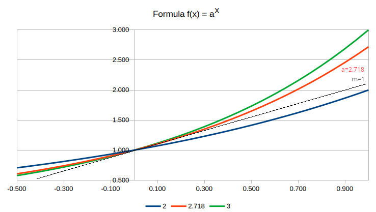
Less intuitive, but if you graph the family of functions y = ax, then solve for 'a' such that the slope at x=0 is equal to 1, then you will calculate Euler's constant (e).
You can start by creating the following table using three values of 'a' (2, 2.718282, and 3).
Table, Family of functions y = ax
| x | a=2 | a=2.718 | a=3 |
|---|---|---|---|
| -0.500 | 0.707 | 0.607 | 0.577 |
| -0.450 | 0.732 | 0.638 | 0.610 |
| -0.400 | 0.758 | 0.670 | 0.644 |
| -0.350 | 0.785 | 0.705 | 0.681 |
| -0.300 | 0.812 | 0.741 | 0.719 |
| -0.250 | 0.841 | 0.779 | 0.760 |
| -0.200 | 0.871 | 0.819 | 0.803 |
| -0.150 | 0.901 | 0.861 | 0.848 |
| -0.100 | 0.933 | 0.905 | 0.896 |
| -0.050 | 0.966 | 0.951 | 0.947 |
| 0.000 | 1.000 | 1.000 | 1.000 |
| 0.050 | 1.035 | 1.051 | 1.056 |
| 0.100 | 1.072 | 1.105 | 1.116 |
| 0.150 | 1.110 | 1.162 | 1.179 |
| 0.200 | 1.149 | 1.221 | 1.246 |
| 0.250 | 1.189 | 1.284 | 1.316 |
| 0.300 | 1.231 | 1.350 | 1.390 |
| 0.350 | 1.275 | 1.419 | 1.469 |
| 0.400 | 1.320 | 1.492 | 1.552 |
| 0.450 | 1.366 | 1.568 | 1.639 |
| 0.500 | 1.414 | 1.649 | 1.732 |
| 0.550 | 1.464 | 1.733 | 1.830 |
| 0.600 | 1.516 | 1.822 | 1.933 |
| 0.650 | 1.569 | 1.916 | 2.042 |
| 0.700 | 1.625 | 2.014 | 2.158 |
| 0.750 | 1.682 | 2.117 | 2.280 |
| 0.800 | 1.741 | 2.226 | 2.408 |
| 0.850 | 1.803 | 2.340 | 2.544 |
| 0.900 | 1.866 | 2.460 | 2.688 |
| 0.950 | 1.932 | 2.586 | 2.840 |
| 1.000 | 2.000 | 2.718 | 3.000 |
Find the slope around 0 for each curve:
Table, Slope (m) at x=0
| a | Δx | Δy | m |
|---|---|---|---|
| 2 | 0.100 | 0.069 | 0.693 |
| 2.718 | 0.100 | 0.100 | 1.000 |
| 3 | 0.100 | 0.110 | 1.099 |
Note: If you were to use a trial and error method, you could adjust 'a' up and down between 2.7 and 2.8 to arrive at the answer of 2.718 such that the slope (m) at x=0 is equal to 1.
Graph
4. Euler's Constant using Differential Calculus
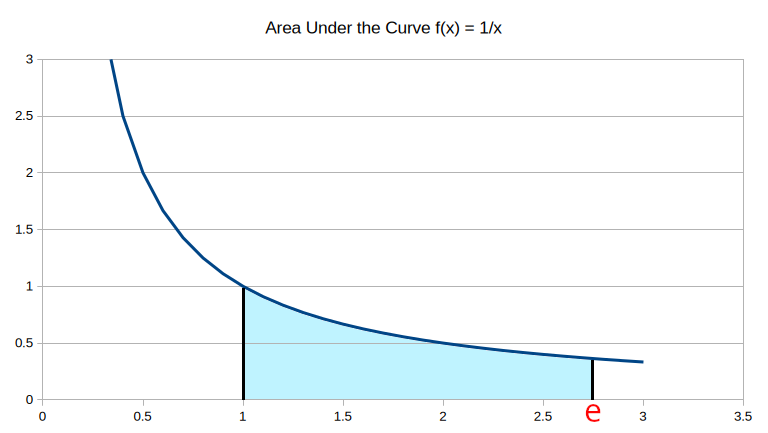
Take the function y = 1/x. Calculate the area under the curve from 1 to 'a' such that the area under the curve is equal to 1. Then a = e = 2.718281.
Expressed as an integral, you have the following function:
To approximate the integral, you can formulate the following table:
Table, Calculating Area under the Curve
| x | f(x) | Δx | An | Sum |
|---|---|---|---|---|
| 1 | 1 | |||
| 1.01 | 0.990 | 0.01 | 0.010 | 0.010 |
| 1.02 | 0.980 | 0.01 | 0.010 | 0.020 |
| 1.03 | 0.971 | 0.01 | 0.010 | 0.029 |
| 1.04 | 0.962 | 0.01 | 0.010 | 0.039 |
| 1.05 | 0.952 | 0.01 | 0.010 | 0.049 |
| ... | ... | ... | ... | ... |
| 2.67 | 0.375 | 0.01 | 0.004 | 0.979 |
| 2.68 | 0.373 | 0.01 | 0.004 | 0.983 |
| 2.69 | 0.372 | 0.01 | 0.004 | 0.986 |
| 2.70 | 0.370 | 0.01 | 0.004 | 0.990 |
| 2.71 | 0.369 | 0.01 | 0.004 | 0.994 |
| 2.72 | 0.368 | 0.01 | 0.004 | 0.997 |
| 2.73 | 0.366 | 0.01 | 0.004 | 1.001 |
| 2.74 | 0.365 | 0.01 | 0.004 | 1.005 |
| 2.75 | 0.364 | 0.01 | 0.004 | 1.008 |
| 2.76 | 0.362 | 0.01 | 0.004 | 1.012 |
| 2.77 | 0.361 | 0.01 | 0.004 | 1.016 |
| 2.78 | 0.360 | 0.01 | 0.004 | 1.019 |
Note: Euler's constant lies between 2.72 and 2.73. e = 2.718.
Graph
If you were to graph the area under the curve, you would have:
5. Compound Interest using Euler's Constant (e)
If you want to take the compound interest of $10,000 over 30 years at a rate of 4.4% per year, then you would use the equation:
f(t) = 10000e0.044t
where:
- f(t) = value in dollars
- e = Euler's constant
- t = time in years
- Principle = $10,000
- Interest = 4.4%
To graph this out, we get the following table:
Table, Compount Interest on $10.000 with Interest of 4.4%
| t | f(t) |
|---|---|
| 0 | $10,000.00 |
| 1 | $10,449.82 |
| 2 | $10,919.88 |
| 3 | $11,411.08 |
| 4 | $11,924.38 |
| 5 | $12,460.77 |
| 6 | $13,021.28 |
| 7 | $13,607.01 |
| 8 | $14,219.09 |
| 9 | $14,858.69 |
| 10 | $15,527.07 |
| 11 | $16,225.52 |
| 12 | $16,955.38 |
| 13 | $17,718.07 |
| 14 | $18,515.07 |
| 15 | $19,347.92 |
| 16 | $20,218.24 |
| 17 | $21,127.70 |
| 18 | $22,078.08 |
| 19 | $23,071.20 |
| 20 | $24,109.00 |
| 21 | $25,193.48 |
| 22 | $26,326.74 |
| 23 | $27,510.98 |
| 24 | $28,748.49 |
| 25 | $30,041.66 |
| 26 | $31,393.00 |
| 27 | $32,805.14 |
| 28 | $34,280.79 |
| 29 | $35,822.82 |
| 30 | $37,434.21 |
Note: at the end of 30 years, you would have $37,434.21 in the bank. Inflation from 1990 to 2018 has averaged around 2.46% per year. You would just be keeping ahead of inflation. $10,000 adjusted for inflation over 30 years at 2.46% would be $22,000. Therefore, you did not make $37,434.21; rather, you made the difference of $37,434.21 and $22,000, or $15,434.21! If you take the ratio, you only increased your wealth by 41%, not the 374% that you thought you made!
The average return on the S&P 500 over the past 30 years, from 1996 to 2025 was 10.4%. If you just purchased an S&P500 index fund and placed your money in the fund, after 30 years you would have $226,463.80: a much better return.
Graphs
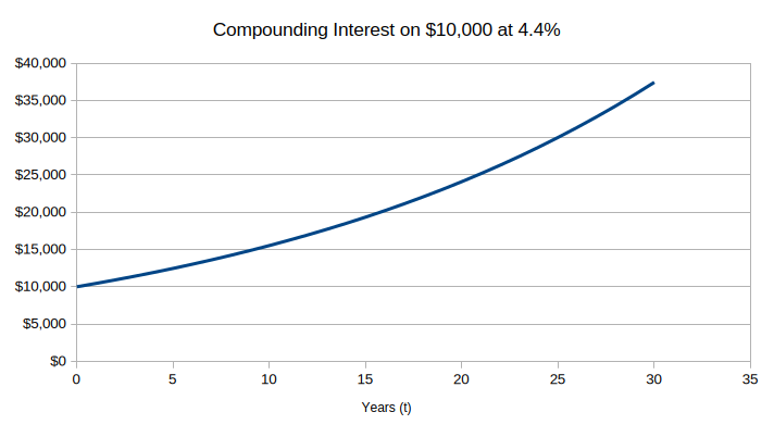
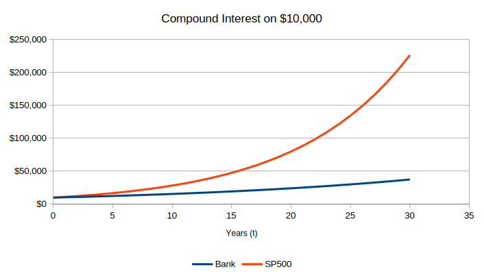
Note: the above graph with money in the bank (blue) looks good until you compare it to the bottom graph which shows the Bank (blue) vs the S&P500 Fund (red curve).
If you were to include a graph of inflation, it would fall somewhere below the blue line.
6. Normal Distribution Curve
Euler's constantant (e) is used in the normal distribution curve using the following equation:
f(x) =
where:
- μ = Mean
- σ = Standard Deviation
Graph
If we draw a graph of f(x) using the above formula, you get the following:
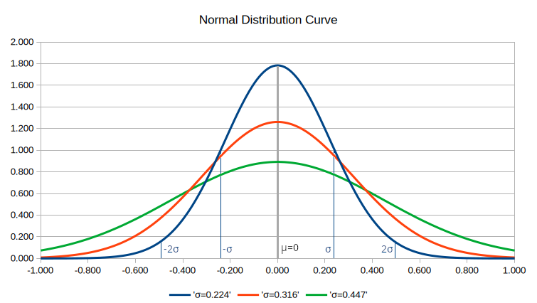
Using the following values:
| Variable | σ=0.224 | σ=0.316 | σ=0.447 | Definition |
|---|---|---|---|---|
| μ | 0 | 0 | 0 | mean |
| σ2 | 0.05 | 0.1 | 0.2 | variance |
| σ | 0.224 | 0.316 | 0.447 | Standard Deviation (SD) |
| 2σ | 0.447 | 0.632 | 0.894 | 2 SD |
The area under the curve for each segment of SD (σ) can be defined by the following table:
| Segment | Area |
|---|---|
| -∞ to -2σ | 2.20% |
| -2σ to -σ | 13.60% |
| -σ to 0 | 34.10% |
| 0 to σ | 34.10% |
| σ to 2σ | 13.60% |
| 2σ to ∞ | 2.20% |
| -1σ to 1σ | 68.20% |
| -2σ to 2σ | 95.40% |
| tails | 4.40% |
Based on this information, if a scientific study defines a population, we say that 95.4% of the data falls within two standard deviations (2SD). This leaves 4.45% of the populations that falls outside this range.
Let us take a study that involves a blood pressure medication. This is defined as a two-tailed test since blood pressure values fall on either side of the mean.
We define two populations: the control group that receives a placebo, and an experimental group that receives the medication. We assume that both groups have been assigned by a randomized method.
These two populations will be represented by their own distribution curves. We define the null hypothesis (Ho) that these two populations are identical. When the study is completed, there will be two normal distributions curves, one for each population. These populations will overlap.
Any separation between the two curves is due to the medication given to the experimental group. The degree of separation determines whether or not the study reaches statistical significance. In this case we say that we failed to prove the null hypothesis (Ho). In a sense, two negatives makes a positive, so conversely, we say that the study had a positive outcome.
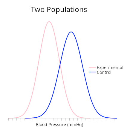
Note: this is the field of Biostatistics, which is outside the scope of this discussion.
top of page